Research Internship · 2023

Neuromorphic Computing and Time-Series Forecasting: Digital Twins of Artificial Spin Ices

Period August – September 2023

Affiliation Blackett Laboratory, Imperial College London

Supervisor Dr Kilian D. Stenning

Responsible Professor Prof. Will R. Branford

Python PyTorch Recurrent Networks Digital Twins Reservoir Computing Physical Neural Networks Time-Series Prediction NumPy

Overview

Conventional AI runs on digital silicon, paying an ever-growing energy cost to parallelise matrix operations. Neuromorphic computing takes a different route: it offloads computation onto the intrinsic physics of a material, using the device's own nonlinear dynamics and memory as the computational substrate. Nanomagnetic artificial spin ices are an attractive candidate — their magnetic microstates provide passive long-term memory, they interact wirelessly through dipolar coupling, and their ferromagnetic-resonance (FMR) spectra expose hundreds of high-dimensional output channels.

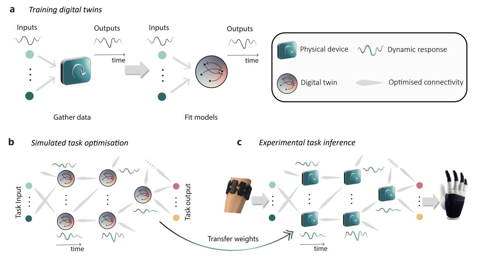
The central challenge is that you cannot run gradient descent directly on a lump of magnetic metamaterial. To optimise a network of physical devices, you first need a differentiable digital twin — a software model that reproduces each device's input–output response closely enough that gradients computed in simulation transfer back to the hardware. During this internship I built the first such twins for the project: recurrent neural networks trained to mimic three distinct nanomagnetic arrays, then combined them in series and parallel architectures and trained the interconnections to forecast the chaotic Mackey–Glass time series.

These preliminary recurrent models established the modelling workflow that was later generalised into the noise-aware neural-SDE framework published in Noise-Aware Training of Neuromorphic Dynamic Device Networks (Manneschi, Vidamour, Stenning, …, Gui, et al., Nature Communications, 2025), on which I am a co-author. The physical-device foundations come from Neuromorphic Few-Shot Learning (Stenning, Gartside, Manneschi, et al., 2024).

Fig. 1 — The dynamical-network optimisation framework: fit differentiable twins to real devices, optimise the interconnections in simulation, then transfer the learned weights back to hardware. *(Manneschi et al., 2025, Nature Communications, Fig. 1.)*

Background: Artificial Spin Ices as Computational Nodes

Why nanomagnets?

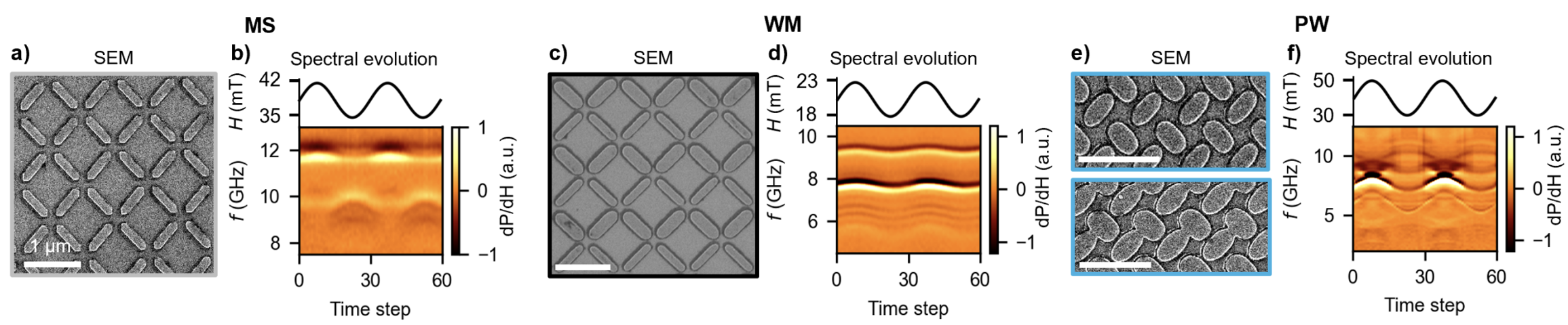
An artificial spin ice is a lithographically patterned array of single-domain nanomagnets. Each bar can sit in a macrospin state (uniformly magnetised) or, in wider bars, collapse into a vortex state. The configuration of the whole array — its microstate — encodes a history-dependent memory of the inputs the device has seen. Because the nanomagnets couple to one another magnetically, the array performs a collective, parallel transformation of its input with no moving charge and minimal waste heat.

The array is read out by ferromagnetic resonance: a swept microwave field excites spin-wave (magnon) modes, and the resulting absorption spectrum acts as a rich, high-dimensional fingerprint of the current microstate. A single array can expose hundreds of frequency-multiplexed output channels, which is exactly the kind of dimensionality reservoir computing thrives on.

The memory–nonlinearity trade-off

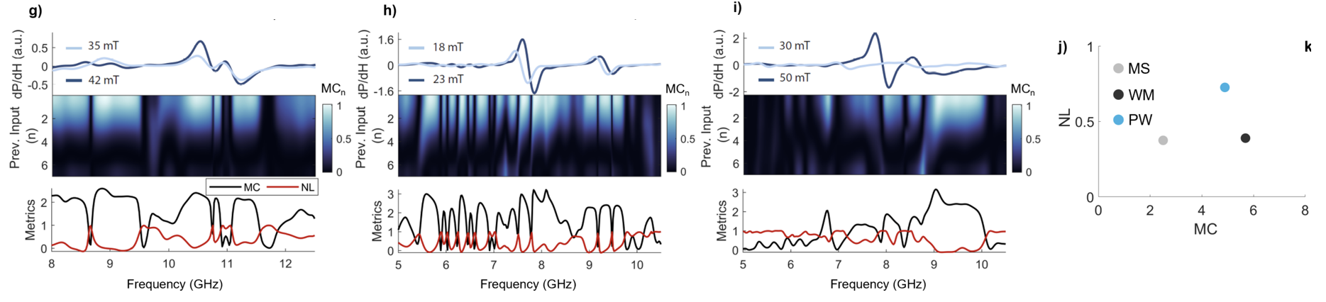
A single physical reservoir faces a fundamental compromise: a system tuned for long memory tends to be weakly nonlinear, and vice versa. This restricts any one device to a narrow band of tasks. The group's strategy is to fabricate several arrays with deliberately different dynamics and wire them together into a multilayer network, so the combined system can supply both high memory and high nonlinearity on demand.

Fig. 2 — The three artificial spin reservoirs. MS supports only macrospins (short memory); WM and PW additionally host vortex states, providing multiple memory timescales and richer nonlinearity. *(Stenning et al., 2024, Fig. 2a–f.)*

The Three Reservoir Arrays

Each array behaves as a distinct "complex node" with its own memory capacity, nonlinearity and output dimensionality. In the digital-twin code each is represented by its own recurrent model, sized to match the array's measured FMR output channels and the temporal depth (look-back) needed to capture its dynamics.

Array	Type	Character	Twin look-back	Output channels
MS	Square artificial spin ice	Macrospin only — short memory	11	375
WM	Width-modified spin-vortex ice	High memory capacity (vortices)	9	201
PW	Pinwheel spin-vortex ice	Highest nonlinearity (disorder)	7	300

The look-back and channel counts above are the values used for the recurrent twins in the training code; they reflect how much temporal context and how many spectral outputs each physical array effectively provides. Quantitatively, each array occupies a different point in the memory-capacity / nonlinearity plane.

Fig. 3 — Memory-capacity and nonlinearity of the three arrays. Vortex-bearing WM/PW reach long memory timescales; PW's disordered microstates give the highest nonlinearity. *(Stenning et al., 2024, Fig. 2g–j.)*

Reservoir Computing with a Single Array

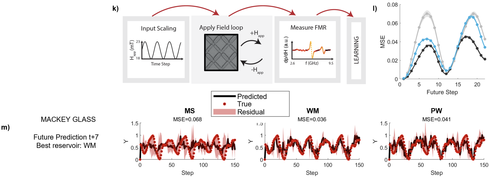
In the single-reservoir scheme, data is encoded as the amplitude of an applied magnetic field loop and the resulting FMR spectrum is read out as the computational output. This works, but a single array hits the memory–nonlinearity ceiling: on the chaotic Mackey–Glass task its forecast quality breaks down periodically and degrades sharply for longer prediction horizons. This is precisely the motivation for connecting arrays into a network.

Fig. 4 — Single-reservoir computing scheme and its Mackey–Glass performance. No single array predicts the chaotic series well across all horizons. *(Stenning et al., 2024, Fig. 2k–m.)*

Building the Digital Twins

Because each array's response depends on the history of inputs, a memoryless model will not do. I modelled each device with a recurrent network (a Gated Recurrent Unit): the input is a sliding window of the driving field amplitude, the recurrent hidden state integrates it over time, and a final linear layer maps the hidden state onto the array's multi-channel FMR output. The data pipeline normalises the Mackey–Glass signal to [0, 1], downsamples it, and reshapes it into overlapping look-back windows.

Each twin learns the map from an input field time-series to the high-dimensional spectral response of one physical array, turning a black-box magnetic device into a differentiable component that gradients can flow through. Trained twins are then frozen, so they act as fixed, faithful surrogates during network optimisation.

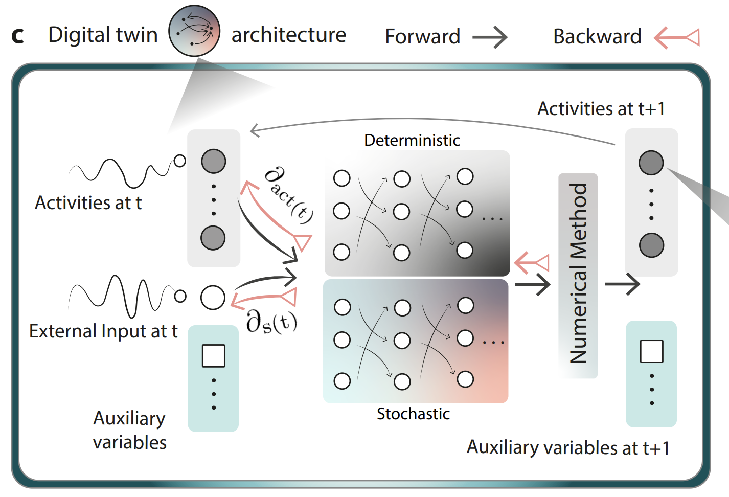
In the published framework this idea is generalised into a neural stochastic differential equation (neural-SDE): paired neural networks model the deterministic dynamics and the stochastic (noise) dynamics, with auxiliary variables capturing coloured noise across multiple timescales, integrated by a numerical SDE solver and trained adversarially.

Fig. 5 — Digital-twin architecture used in the published framework: a deterministic network (upper) and a stochastic network (lower) jointly predict each device's next state. My recurrent twins were the deterministic precursor to this design. *(Manneschi et al., 2025, Nature Communications, Fig. 2c.)*

Combining Twins into a Physical Neural Network

With differentiable twins in hand, I assembled them into larger networks that mirror how the physical arrays are wired together. Two combination schemes were implemented:

Series combination

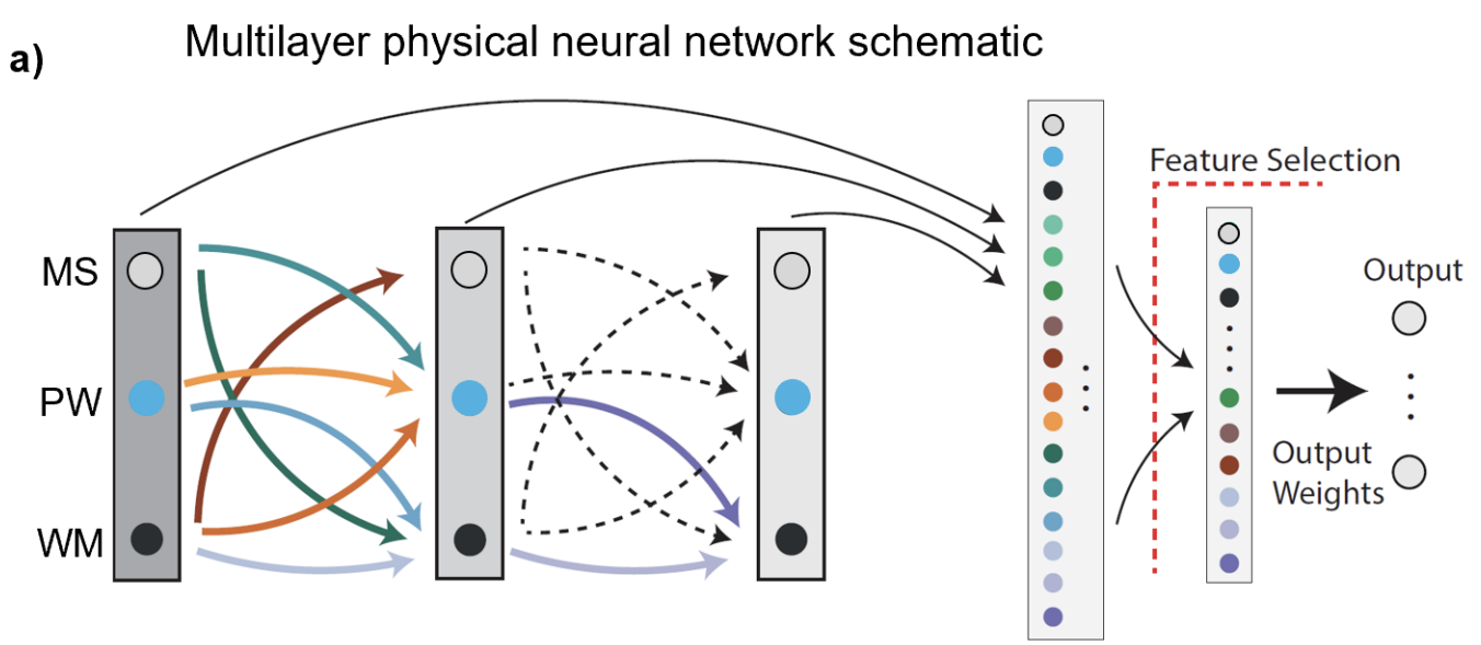
The output channels of one array are collapsed into a single driving signal for the next array through a trainable interconnection weight (followed by a sigmoid to keep the signal in the device's responsive field range). This is the software analogue of the programmable interconnects between physical nodes. Two- and three-layer series networks were supported (e.g. MS → WM → PW), with the states from every layer concatenated and fed to a final read-out layer.

Parallel combination

Several twins receive the same input and their output states are concatenated, with no information passing between nodes — boosting dimensionality but not memory. Comparing series against parallel makes explicit how much the inter-node connectivity contributes.

Only the interconnection and read-out weights are trained; the device twins stay frozen. This is precisely the physical-neural-network paradigm — optimise the connectivity, not the devices — implemented entirely in a differentiable simulation.

Fig. 6 — Multilayer physical neural network built from the arrays as complex nodes, combined in series and parallel. *(Stenning et al., 2024, Fig. 3a.)*

Task & Training: Mackey–Glass Forecasting

The benchmark is the Mackey–Glass delay-differential system, a standard chaotic time-series prediction task whose quasi-periodic dynamics demand both memory and nonlinearity. The network was trained to predict the signal multiple steps into the future simultaneously — twenty future horizons (t+1 … t+20) at once — so a single read-out layer must capture the full forecast profile.

Hyper-parameter	Value
Optimiser	Adam
Learning rate	0.001
Epochs	500
Loss	Mean-squared error (MSE)
Future horizons	20 (t+1 … t+20)
Train / test split	600 / 300 samples

Results

Connectivity beats single arrays

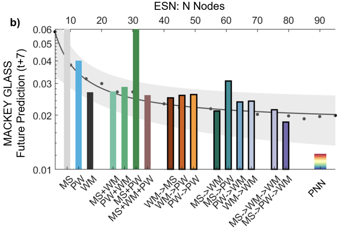
Comparing single twins, parallel combinations and full series/multilayer networks quantifies the benefit of inter-node connectivity. The networked architectures substantially outperform any single array, and the ordering of arrays (from low to high memory) matters.

Fig. 7 — Forecasting MSE across architectures: the multilayer network beats every single array and parallel combination. *(Stenning et al., 2024, Fig. 3b.)*

Forecast accuracy vs prediction horizon

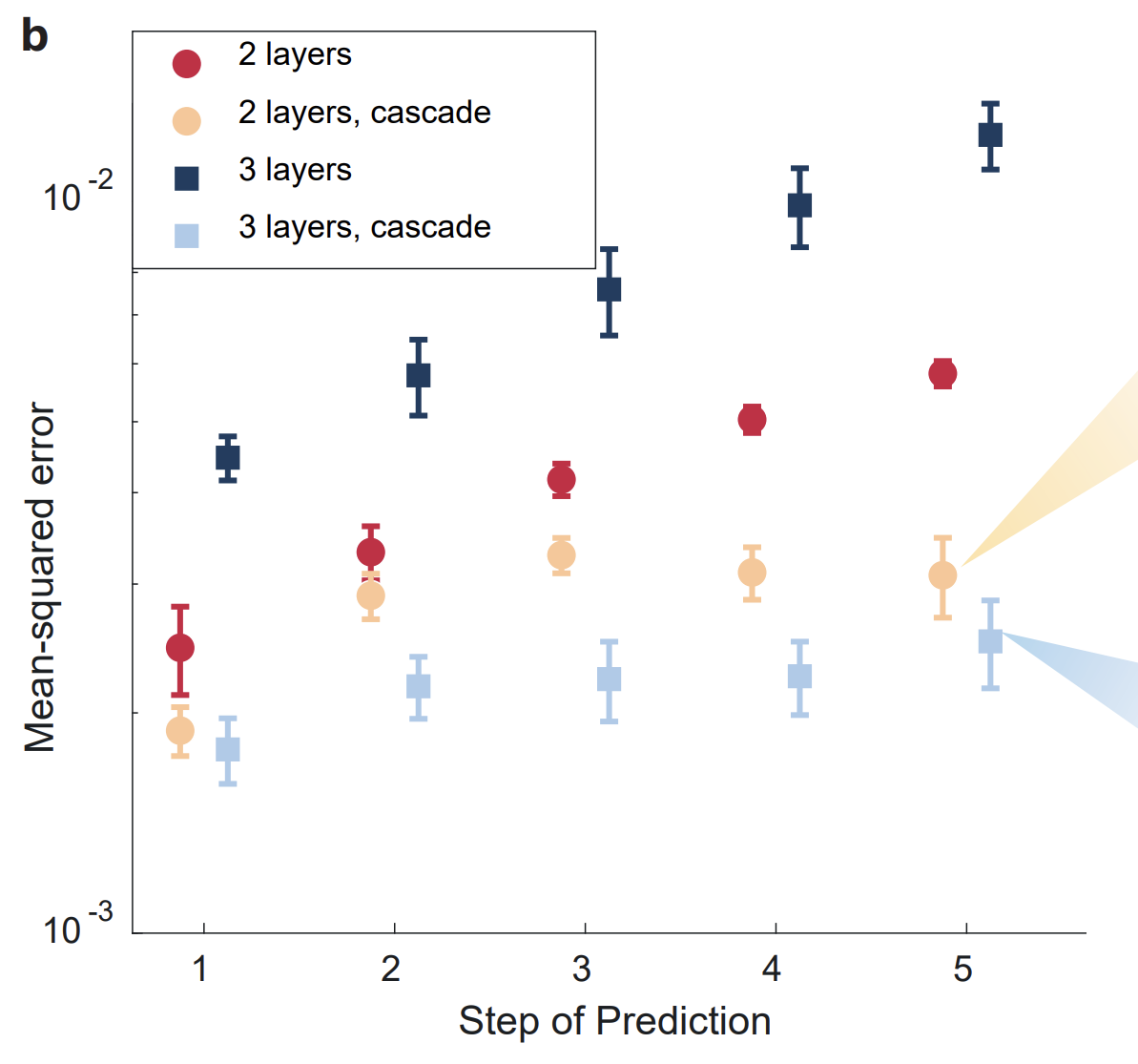
As expected for a chaotic system, error grows with how far ahead the network is asked to predict. Cascade learning — training the layers sequentially with intermediate hardware data — keeps the error low as more layers (and longer horizons) are added.

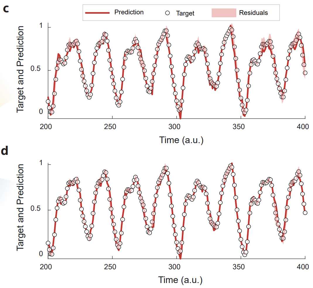
Fig. 8 — Mean-squared error versus prediction horizon for transferred networks; cascade learning gives the best, most scalable performance. *(Manneschi et al., 2025, Nature Communications, Fig. 4b.)*

Predicted vs target signal

Overlaying the network's forecast on the ground-truth Mackey–Glass trace shows how faithfully the physical-twin network reconstructs the chaotic dynamics.

Fig. 9 — Predicted versus target Mackey–Glass signal for the transferred network. *(Manneschi et al., 2025, Nature Communications, Fig. 4c–d.)*

Why Noise Matters: From Preliminary Twins to the Published Framework

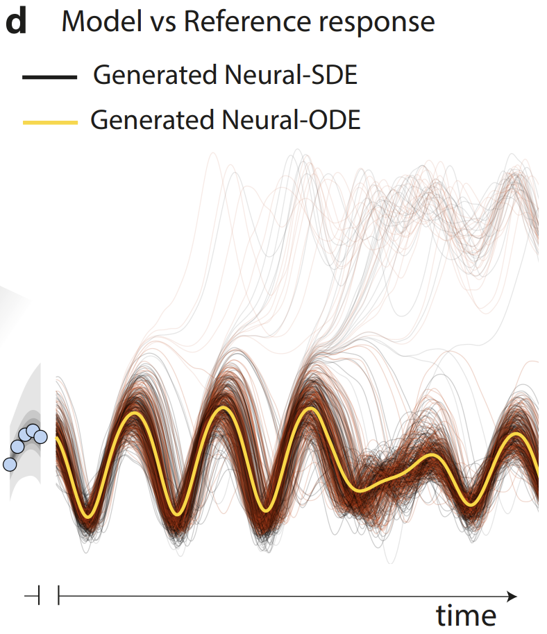
These recurrent twins were the project's first working device models, and they exposed a key limitation: a purely deterministic model captures the average response of an array but not its noise. Real nanomagnetic devices show stochastic, noise-induced bifurcations, and a noise-free twin leads networks to settle on connectivity that looks excellent in simulation but degrades once transferred to hardware.

The published paper resolves this by replacing the deterministic twins with neural-SDEs that model both deterministic dynamics and coloured noise, trained adversarially and optimised through backpropagation-through-time and cascade learning. A deterministic neural-ODE collapses every run to a single trajectory; the neural-SDE instead reproduces the full distribution of device responses — including the bifurcations the noise-free model misses.

Fig. 10 — Why noise awareness matters: the deterministic neural-ODE gives one trajectory, while the neural-SDE captures the experimentally observed spread and noise-induced bifurcations. *(Manneschi et al., 2025, Nature Communications, Fig. 2d.)*

Author contribution (from the published paper): the preliminary recurrent models for the spin-ice devices were developed by K. D. Stenning, L. Gui, D. Sonawala and D. Donskikh — the work this page describes.

Summary

Differentiable device twins: Built recurrent models that reproduce the high-dimensional FMR response of three distinct nanomagnetic arrays (MS, WM, PW), turning black-box magnetic devices into gradient-friendly components.

Physical neural networks in simulation: Combined the frozen twins into series and parallel architectures with trainable interconnections, and trained them to forecast the chaotic Mackey–Glass series over 20 future horizons.

Foundation for the published work: Established the digital-twin + network-combination workflow that was generalised into the noise-aware neural-SDE (Stochastic Differential Equation) framework published in Nature Communications in 2025, on which I am a co-author.

This internship was my first deep exposure to treating physics as a computational resource — designing models whose gradients are meant to cross the simulation-to-hardware gap. The same instinct, finding faithful differentiable surrogates for messy physical systems, runs through my later detector-simulation and quantitative work.

All Research